Practical cases
In this chapter, a number of practical cases is shown to exemplify most of the concepts explained in the previous chapters. Links to the relevant parts of this manual are provided when applicable for the interested reader. Bear in mind that this tutorial does not cover all the possibilities offered by the software developed at the Seventh International Competition. Therefore, referring to the manual pages is a good idea to get a detailed picture of all the possibilities.
In the first example, the temporal satisficing planners yahsp2 and its multithreaded version yahsp2-mt are evaluated in two domains: crewplanning and turnandopen. None of these planners is known to have any particular requirement —however, it will be shown that they can be easily identified and met when following the procedure depicted below.
The second example shows how to set-up the environment for running experiments with the software developed at the Seventh International Planning Competition. This example has been explicitly created to encourage users to use this software for evaluating their own planners —though official entries of the Seventh International Planning Competition have been chosen to allow reproducibility. In particular, the planner probe and the domain openstacks are used here.
The third example shows how to compare the performance of a particular planner with the performance of other planners that entered the Seventh International Planning Competition. Here, the planner probe will be compared in the opestacks domain to the performance of the winner of the Sequential Satisficing (seq-sat) track lama-2011.
The fourth example discusses how to perform a statistical test to derive accurate figures about the relative performance of two planners on the same problem. In this case, the planners yahsp2 and its multithreaded version yahsp2-mt are used with problem 001 of the domain openstacks.
Readers are strongly encouraged to follow the examples in the same order they are given here: while the main goal of the first practical case is to show how to run particular experiments with planners and domains stored in a particular svn server and how to inspect the resulting data, the second and third practical cases are intended to show how to set-up their own svn servers and perform comparisons with the performance of entrants of the Seventh International Planning Competition —and, in general, to any other planner.
First practical case
In this example, the temporal satisficing planners yahsp2 and its multithreaded version yahsp2-mt are evaluated in two domains: crewplanning and turnandopen. None of these planners is known to have any particular requirement —however, it will be shown that they can be easily identified and met when following the procedure depicted here.
The time limit will be set to 10 seconds so that this tutorial can be run without waiting too long for the results. Besides, the memory limit will be set to 2 Gb which is rather typical in most modern computer configurations.
It is assumed that this exercise is performed in the same machine where the results are about to be stored and examined. Nevertheless, nothing prevents experienced users to run the experiments in remote computers using ssh commands provided that they retrieve the result directories as explained in The results directory. However, this topic is not covered here.
The tutorial is divided in the following parts:
Setting up: A linux computer is configured to meet all the dependencies of the IPC software; next, the software is installed in a single command and the INI configuration file is created Running: The competition is run for the abovementioned planners and domains. The time limit is 10 seconds and the memory bound is set to 2 Gb —which is assumed to be a minimum in modern computer configurations. Reporting: The results are examined. First a snapshot is created and then various reports are created to show how different values can be retrieved in a wide variety of formats. Finally, the score sheet used at the International Planning Competition is used to rank planners.
In those cases where the output is intentionally ommitted an ellipsis is inserted instead.
Setting up
The first step consists of configuring a computer to run the experiments and to examine the results. While it is not necessary at all that both tasks are performed in the same computer, this is not discussed here since it goes beyond the scope of this document. However, experienced users will have no trouble in getting this done. As a matter of fact, that was actually the layout during the Seventh International Planning Competition.
It is assumed as well, that users have privileges to install software. If not, contact your system administrator or install them in your account.
In this example, GNU/Linux Ubuntu 11.04 has been installed in a computer —as a matter of fact, the experiments were run on a VMWare Virtual Machine with 2Gb of RAM. Of course, python 2.7 and svn have to be available in the computer as well as the software required by the selected planners to be built. While Python 2.7 is available by default in the latest version of GNU/Linux at the time of writing this manual, this does not apply to subversion. Therefore, to download and install svn:
$ sudo apt-get install subversion
In any case, before moving on make sure that both Python 2.7 and subversion are available in your computer:
$ python --version
$ svn --version
If they are, the previous commands shall report the current versions installed in your machine.
Since we want to use the software developed at the Seventh International Planning Competition in its full glory, all the dependencies of all modules shall be met before moving on:
- The package IPCData have dependencies with the Python packages ConfigObj and Subversion Python as explained in Dependencies
- The package IPCReport has a single dependency with the Python package pyExcelerator as discussed in Dependencies
- Finally, both packages use the PrettyTable module which is distributed separately
As soon as they are all available, the software of the Seventh International Planning Competition can be checked out from the official repository (or any other one of your choice provided that you have a private copy) and configured accordingly before running the experiments. All of these steps are described in detail in the following subsections.
ConfigObj
In its authors’ words: ConfigObj is a simple but powerful config file reader and writer: an ini file round tripper. Its main feature is that it is very easy to use, with a straightforward programmer’s interface and a simple syntax for config files [1].
The tarball configobj.zip is downloaded from http://www.voidspace.org.uk/python/configobj.html and unzipped in a temporary directory [2]. Next, the installation process is invoked with the script setup.py:
$ unzip configobj.zip
  ...
$ cd configobj-4.7.2
$ sudo python ./setup.py install
Subversion Python
According to the authors: The pysvn project’s goal is to enable tools to be written in Python that use Subversion [3], such as the IPCData package developed for the Seventh International Planning Competition.
This package is distributed also as an Ubuntu package. Therefore, the installation process consists simply of executing:
$ sudo apt-get install python-svn
pyExcelerator
The pyExcelerator Python package allows the creation of Excel worksheets with various features including decorators, splitters, etc.
As it turned out with ConfigObj, it is necessary to download the tarball and to install it. The whole process is performed in a temporary directory:
$ unzip pyexcelerator-0.6.4.1.zip
  ...
$ cd pyexcelerator-0.6.4.1
$ sudo python ./setup.py install
And pyExcelerator is available in the computer [4].
NumPy and SciPy
The installation instructions of NumPy and SciPy (that cover various platforms) provide a step by step procedure to install the software form the source code. However, in a Linux box it is easier just to install the apt packages as follows:
$ sudo apt-get install python-numpy
  ...
$ sudo apt-get install python-scipy
  ...
prettyTable
In its authors’ words: PrettyTable is a simple Python library designed to make it quick and easy to represent tabular data in visually appealing ASCII tables.
To use this software it suffices going to the Donwload area in the project homepage and to get the file PrettyTable.py. Nevertheless, this is not necessary at all since it is automatically included in the packages developed at the Seventh International Planning Competition.
Downloading the IPC Software
The software of the IPC can be easily retrieved from the official svn server of the Seventh International Planning Competition. Make sure, first, to move to an empty ancilliary directory:
$ cd ~/tmp
$ mkdir first-case
$ cd first-case
$ svn co svn://svn@pleiades.plg.inf.uc3m.es/ipc2011/data/scripts/pycentral
Upon completion, all modules IPCData, IPCReport, IPCPrivate and IPCTools are checked out and located in the directory pycentral that is beneath the current directory.
Configuring the IPC Software
As a matter of fact, there is no need to configure the IPC software unless automatic e-mail notification is desired —for a thorough discussion on the topic visit seed.py. However, even if this feature is not going to be used, it might be a good idea to start by running the script seed.py since it automatically browses the contents of the svn server to be used and issues a number of warnings if some track/subtracks are found empty. In this example, the svn server chosen is:
svn://svn@pleiades.plg.inf.uc3m.es/ipc2011/data
but it could be an arbitrary one [5].
Since this script is located in the package IPCData we move there to execute it:
$ cd pycentral/IPCData
$ ./seed.py --file ~/.ipc.ini --name "A practical case" --part "Deterministic Part"
            --bookmark svn://svn@pleiades.plg.inf.uc3m.es/ipc2011/data
            --wiki http://www.plg.inf.uc3m.es/ipc2011-deterministic
            --cluster pleiades.plg.inf.uc3m.es
            --mailuser ipc2011.pleaides@gmail.com --mailpwd ys98NfyMenRs
            --smtp smtp.gmail.com --port 587
All the parameters are mandatory though most of them are almost never used. However, --mailuser, --mailpwd, smtp and port are mandatory if the automatic notification by e-mail is desired when running any of the following scripts: invokeplanner.py, builddomain.py, buildplanner.py or validate.py. Besides, if the INI configuration file is created there is no need to specify the svn bookmark anymore in any command that requires it since doing it just overrides the default selection specified in the INI configuration file. By default, all scripts seek the INI configuration file in ~/.ipc.ini.
Finally, the INI configuration file just created contains a detailed explanation of the contents of the svn server which are self-explanatory.
Running
All the previous steps take less than 10 minutes in a computer with a standard connection to Internet. Now, the environment is set up for starting any execution. In what follows, all scripts but check.py are exemplified —this script is only suitable for arranging an official competition and serve to very particular goals, see check.py.
First, the competition will be run automatically but before that, it is shown how the domains and planners are checked out and compiled. Next, it will be shown how to validate the results.
In general, as it will be shown, the main driver behind the design of the IPC software is to hide the contents and design of the svn server to the user. Only people interested in adding planners and/or domains shall be involved with the contents of the svn server.
Building domains
Users interested in just downloading a number of domains to their computer will find builddomain.py handy. In our running example the temporal satisficing domains crewplanning and turnandopen have been selected. To download them:
 $ ./builddomain.py --track tempo --subtrack sat
                    --domain crewplanning turnandopen --directory ~/tmp

[Info: using the svn bookmark specified in the ipc ini configuration file]
[      svn://svn@pleiades.plg.inf.uc3m.es/ipc2011/data]


[Info: the following domains have been built]
[      [u'crewplanning', u'turnandopen']]
First, note that the svn bookmark has not been specified. Indeed, an info message informs that the default selection found in ~/.ipc.ini is about to be used. Finally, another info message informs that the desired domains have been properly built. As specified with the directive --directory, both domains have been built under ~/tmp —if no directory is specified, the domains are built under the current directory. The reader is invited to examine the contents of ~/tmp/crewplanning and ~/tmp/turnandopen. As it can be seen, both directories consist of a number of testsets that contains pairs of PDDL domain and problem files.
Building planners
However, most people might find it even more useful just to download and compile particular planners. This is done with the module buildplanner.py. In our running example, the planner selected is yahsp2. Thus, the following command automates all the necessary tasks:
 $ ./buildplanner.py --track tempo --subtrack sat
                    --planner yahsp2 yahsp2-mt --directory ~/tmp

[Info: using the svn bookmark specified in the ipc ini configuration file]
[      svn://svn@pleiades.plg.inf.uc3m.es/ipc2011/data]


[Info: the following planners have been built]
[      [u'yahsp2', u'yahsp2-mt']]
This command explicitly requests downloading all the software of the temporal satisficing planners yahsp2 and yahsp2-mt [6]. Since no svn bookmark has been specified with the directive --bookmark, it is automatically retrieved from the INI configuration file ~/.ipc.ini as reported in the first info message [7]. Finally, the building process of the selected planners finishes and this is reported in the last info message.
Upon completion, the reader is invited to check the contents of the directories ~/tmp/yahsp2 and ~/tmp/yahsp2-mt. There are two files of particular interest build-yahsp2.log and build-yahsp2-mt.log [8]. These files record the output of all the building process. A quick examination of their contents reveals that this software needs the GNU Multiple Precision library and the flex and bison utilities [9]. To install them:
$ sudo apt-get install libgmp3-dev
$ sudo apt-get install bison
$ sudo apt-get install flex
Now, before trying to rebuild both planners make sure that the target directories are empty:
$ rm -rf ~/tmp/yahsp2*
And now issue the same command shown above to build the planners.
Automating the whole process
In general, most users will use this software to automate both tasks: downloading a particular set of domains and build a particular set of planners and to run the planner in all the testsets generated so far. The results shall be stored in a directory which follows the design of a results directory —see The results directory. All of these tasks are automated with the script invokeplanner.py which uses the previous services. In addition it automates the execution of the planners and stores the results in a particular order as mentioned earlier. Finally, if requested (as in our running example), it sends an automatic e-mail with the log file generated during the whole process.
In case the reader followed the two previous sections, make sure to remove all the directories that contain the planners and domains since invokeplanner.py will attempt to create the same directories. If they exist, an error message will be issued and the script resumes execution:
$ rm -rf ~/tmp/yahsp2*
$ rm -rf ~/tmp/crewplanning
$ rm -rf ~/tmp/turnandopen
Now, the following command starts the whole process:
$ ./invokeplanner.py --track tempo --subtrack sat --planner 'yahsp2*'
                     --domain crewplanning turnandopen
                     --directory ~/tmp --logfile tutorial
                     --email carlos.linares@uc3m.es --timeout 10 --memory 2
First, note that the script uses much the same directives that are acknowledged by both buildplanner.py and builddomain.py. In fact they have the same purpose. Other directives which are new in invokeplanner.py include:
--logfile This flag requests the script to record the log of all the process in a separate logfile. Since there might be different logfiles that result from different invocations of invokeplanner.py the current date and time is appended to the name provided. If an e-mail account was set-up in the INI configuration file, it is allowed now to instruct invokeplanner.py to send a copy of the logfile generated to a number of recipients. --timeout, --memory set the computational resources available. Time is measured in seconds and memory in Gigabytes. If any of these limits is exceeded, the script automatically kills the planner and all of its children, if any.
Upon completion, the script leaves in the directory ~/tmp/results the results of all the experiments. For a thorough discussion of the purpose and contents of each file generated see invokeplanner.py. All the other directories can be safely removed if desired.
Finally, an automatic message gets to the inbox of the specified recipients. Among other important messages, a summary of the results is provided at the bottom. More importantly, the following table reports the number of problems solved so far:
 * Number of solved instances:
+-----------+--------------+-------------+-------+
| *         | crewplanning | turnandopen | total |
+-----------+--------------+-------------+-------+
| yahsp2    |      20      |      19     |   39  |
| yahsp2-mt |      20      |      19     |   39  |
| total     |      40      |      38     |       |
+-----------+--------------+-------------+-------+
As it can be seen, the planner reports that all planning tasks but one have been solved. If a logfile was requested when invoking invokeplanner.py, it is attached to the automated e-mail as well. For a discussion of the information contained in the log file see The results directory.
Validating the results
Since all planners are expected to generate plans in a format recognizable by VAL it makes sense to check the validity of all plans generated so far. Since version 1.1 of the software of the Seventh International Planning Competition the version used is VAL-4.2.09 and it can be downloaded from http://www.plg.inf.uc3m.es/ipc2011-deterministic/FrontPage/Software
Before moving on, download this software and install it in your computer as follows:
$ tar zxvf VAL-4.2.09.tar.gz
  ...
$ cd VAL-4.2.09
$ make
make sure to add the path to the resulting executable validate in your .cshrc or .bashrc configuration files so that they can be executed from any location.
Now, from the directory where the module IPCData is located use the script validate.py (see validate.py) as follows:
$ ./validate.py --directory ~/tmp/results
  ...

  +---------------+----------+------------------+--------------------+
  | # directories | # solved | # solution files | # successful plans |
  +---------------+----------+------------------+--------------------+
  |       80      |    40    |       309        |         60         |
  +---------------+----------+------------------+--------------------+
This script automatically traverses the results directory and applies the VAL tool to all planning tasks. It then leaves a validation log file in each directory visited. As a result it prints out the summary shown above:
directories: informs about the number of directories visited. Since there were two planners running twenty different cases from two different domains, there were 80 directories in total. solved: is the number of plans that have been properly validated. From here it resuls that half of them where either not generated or invalid. solution files: is the total number of plan solution files generated. There were in total up to 309 plan.soln files generated —for more information on these files see invokeplanner.py. Clearly there were a number of planning tasks that got many solutions. successful plans: only 60 out of the 309 plan solution files generated so far were valid. All the rest being invalid.
Reporting
Once the results have been generated, it is feasible now to inspect them. This is accomplished with the package IPCReport.py —see IPCReport. It serves not only to inspect the values of particular variables, but also to rank the performance of all the planners at any time within the current limit and also to study how the score of each planner evolves over time. All of these steps are examined in detail in the following subsections.
In the next sections it is assumed that the results directory generated in the previuos section has been moved to another computer with all the necessary facilities (mainly LibreOffice or OpenOffice and a full installation of the LaTeX packages) or that they are available in the same computer where all the previous experimentation was conducted.
Inspecting variables
The module report.py (see report.py) provides a clean interface to access the values of a large number of variables. For a complete list of all the variables acknowledge by report.py see Reporting variables or use the command-line argument --variables. In the following, a number of examples of its usage are shown.
It would be natural to start wondering what plan solution files were valid and which were not in the previous example. The following command returns a summary of the total number of problems, the total number of problems that are claimed to have been solved by each planner and the total number of problems that have been properly validated:
$ ./report.py --directory ~/tmp/results/tempo-sat --variable numprobs numsolved oknumsolved

  ...

name: report
+----------+-----------+-------------+
| numprobs | numsolved | oknumsolved |
+----------+-----------+-------------+
|    80    |     78    |      40     |
+----------+-----------+-------------+
legend:
  numprobs: total number of problems [elaborated data]
  numsolved: number of solved problems (independently of the solution files generated)
             [elaborated data]
  oknumsolved: number of *successfully* solved problems (independently of the solution
               files generated) [elaborated data]

created by IPCrun 1.2 (Revision: 295), Fri Oct  7 15:54:05 2011
This information, obtained in a different way, is consistent with the information reported by the logfile sent by invokeplanner.py and the summary provided by the validate.py module. Note that the directory provided this time is ~/tmp/results/tempo-sat. When using the reporting tools it is mandatory to provide the root of the track/subtrack and not the root of the results tree.
To get a detailed picture of what really goes on in each particular case:
$ ./report.py --directory ~/tmp/results/tempo-sat --variable numsols oknumsols

  ...

name: report
+-----------+--------------+---------+---------+-----------+
|  planner  |    domain    | problem | numsols | oknumsols |
+-----------+--------------+---------+---------+-----------+
|   yahsp2  | crewplanning |   000   |    1    |     1     |
|   yahsp2  | crewplanning |   001   |    1    |     1     |
|   yahsp2  | crewplanning |   002   |    1    |     1     |
|   yahsp2  | crewplanning |   003   |    2    |     2     |
|   yahsp2  | crewplanning |   004   |    2    |     2     |
|   yahsp2  | crewplanning |   005   |    1    |     1     |
|   yahsp2  | crewplanning |   006   |    1    |     1     |
|   yahsp2  | crewplanning |   007   |    1    |     1     |
|   yahsp2  | crewplanning |   008   |    1    |     1     |
|   yahsp2  | crewplanning |   009   |    1    |     1     |
|   yahsp2  | crewplanning |   010   |    3    |     3     |
|   yahsp2  | crewplanning |   011   |    3    |     3     |
|   yahsp2  | crewplanning |   012   |    1    |     1     |
|   yahsp2  | crewplanning |   013   |    1    |     1     |
|   yahsp2  | crewplanning |   014   |    1    |     1     |
|   yahsp2  | crewplanning |   015   |    1    |     1     |
|   yahsp2  | crewplanning |   016   |    1    |     1     |
|   yahsp2  | crewplanning |   017   |    1    |     1     |
|   yahsp2  | crewplanning |   018   |    1    |     1     |
|   yahsp2  | crewplanning |   019   |    3    |     3     |
|   yahsp2  | turnandopen  |   000   |    6    |     0     |
|   yahsp2  | turnandopen  |   001   |    2    |     0     |
|   yahsp2  | turnandopen  |   002   |    6    |     0     |
|   yahsp2  | turnandopen  |   003   |    3    |     0     |
|   yahsp2  | turnandopen  |   004   |    7    |     0     |
|   yahsp2  | turnandopen  |   005   |    11   |     0     |
|   yahsp2  | turnandopen  |   006   |    5    |     0     |
|   yahsp2  | turnandopen  |   007   |    9    |     0     |
|   yahsp2  | turnandopen  |   008   |    8    |     0     |
|   yahsp2  | turnandopen  |   009   |    4    |     0     |
|   yahsp2  | turnandopen  |   010   |    3    |     0     |
|   yahsp2  | turnandopen  |   011   |    0    |     0     |
|   yahsp2  | turnandopen  |   012   |    7    |     0     |
|   yahsp2  | turnandopen  |   013   |    5    |     0     |
|   yahsp2  | turnandopen  |   014   |    10   |     0     |
|   yahsp2  | turnandopen  |   015   |    2    |     0     |
|   yahsp2  | turnandopen  |   016   |    11   |     0     |
|   yahsp2  | turnandopen  |   017   |    5    |     0     |
|   yahsp2  | turnandopen  |   018   |    7    |     0     |
|   yahsp2  | turnandopen  |   019   |    5    |     0     |
| yahsp2-mt | crewplanning |   000   |    1    |     1     |
| yahsp2-mt | crewplanning |   001   |    1    |     1     |
| yahsp2-mt | crewplanning |   002   |    1    |     1     |
| yahsp2-mt | crewplanning |   003   |    4    |     4     |
| yahsp2-mt | crewplanning |   004   |    4    |     4     |
| yahsp2-mt | crewplanning |   005   |    1    |     1     |
| yahsp2-mt | crewplanning |   006   |    1    |     1     |
| yahsp2-mt | crewplanning |   007   |    1    |     1     |
| yahsp2-mt | crewplanning |   008   |    1    |     1     |
| yahsp2-mt | crewplanning |   009   |    1    |     1     |
| yahsp2-mt | crewplanning |   010   |    3    |     3     |
| yahsp2-mt | crewplanning |   011   |    3    |     3     |
| yahsp2-mt | crewplanning |   012   |    1    |     1     |
| yahsp2-mt | crewplanning |   013   |    1    |     1     |
| yahsp2-mt | crewplanning |   014   |    1    |     1     |
| yahsp2-mt | crewplanning |   015   |    1    |     1     |
| yahsp2-mt | crewplanning |   016   |    1    |     1     |
| yahsp2-mt | crewplanning |   017   |    1    |     1     |
| yahsp2-mt | crewplanning |   018   |    1    |     1     |
| yahsp2-mt | crewplanning |   019   |    3    |     3     |
| yahsp2-mt | turnandopen  |   000   |    23   |     0     |
| yahsp2-mt | turnandopen  |   001   |    3    |     0     |
| yahsp2-mt | turnandopen  |   002   |    11   |     0     |
| yahsp2-mt | turnandopen  |   003   |    3    |     0     |
| yahsp2-mt | turnandopen  |   004   |    5    |     0     |
| yahsp2-mt | turnandopen  |   005   |    7    |     0     |
| yahsp2-mt | turnandopen  |   006   |    3    |     0     |
| yahsp2-mt | turnandopen  |   007   |    3    |     0     |
| yahsp2-mt | turnandopen  |   008   |    1    |     0     |
| yahsp2-mt | turnandopen  |   009   |    1    |     0     |
| yahsp2-mt | turnandopen  |   010   |    1    |     0     |
| yahsp2-mt | turnandopen  |   011   |    0    |     0     |
| yahsp2-mt | turnandopen  |   012   |    11   |     0     |
| yahsp2-mt | turnandopen  |   013   |    8    |     0     |
| yahsp2-mt | turnandopen  |   014   |    12   |     0     |
| yahsp2-mt | turnandopen  |   015   |    12   |     0     |
| yahsp2-mt | turnandopen  |   016   |    6    |     0     |
| yahsp2-mt | turnandopen  |   017   |    9    |     0     |
| yahsp2-mt | turnandopen  |   018   |    11   |     0     |
| yahsp2-mt | turnandopen  |   019   |    3    |     0     |
+-----------+--------------+---------+---------+-----------+
legend:
  planner [key]
  domain [key]
  problem [key]
  numsols: total number of solution files generated [raw data]
  oknumsols: total number of *successful* solution files generated [raw data]

created by IPCrun 1.2 (Revision: 295), Fri Oct  7 15:58:09 2011
This command reports the number of plan solution files generated and how many of them were valid. As specified in the logfile sent by invokeplanner.py both planners failed to solve a particular instance of the domain turnandopen. This instance is 011. Besides, though both planners generated a number of plan solution files in the turnandopen domain, none is valid.
Whether both planners failed on time or memory or due to any other reason can be queried also:
$ ./report.py --directory ~/tmp/results/tempo-sat
              --variable numfails timefails memfails unexfails

  ...

name: report
+----------+----------------+----------+-----------+
| numfails |   timefails    | memfails | unexfails |
+----------+----------------+----------+-----------+
|    2     | ['011', '011'] |    []    |     []    |
+----------+----------------+----------+-----------+
legend:
  numfails: total number of fails [elaborated data]
  timefails: problem ids where the planner failed on time [elaborated data]
  memfails: problem ids where the planner failed on memory [elaborated data]
  unexfails: problem ids where the planner unexpectedly failed [elaborated data]

created by IPCrun 1.2 (Revision: 295), Fri Oct  7 16:03:57 2011
As it can be seen, both planners could not solve problem 011 in the given time limit so that they were killed after the time bound (10 seconds) was reached.
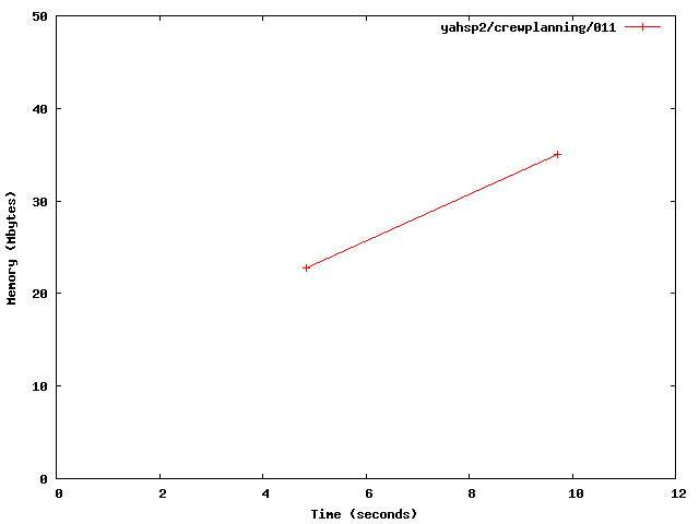
It is also feasible to examine the performance of the planner from a different point of view. For example, to examine the memory profile of the planner when solving a particular problem. Take problem 011 of the crewplanning domain and examine the memory usage of yahsp2:
$ ./report.py --directory ~/tmp/results/tempo-sat
              --variable timelabels memlabels --unroll
              --planner 'yahsp2$' --domain crewplanning --problem 011

  ...

name: report
+-----------+--------------+---------+------------+-----------+
|  planner  |    domain    | problem | timelabels | memlabels |
+-----------+--------------+---------+------------+-----------+
|   yahsp2  | crewplanning |   011   |    4.84    |   22.72   |
|   yahsp2  | crewplanning |   011   |    9.72    |   34.97   |
+-----------+--------------+---------+------------+-----------+
legend:
  planner [key]
  domain [key]
  problem [key]
  timelabels: time ticks used for sampling memory consumption (in seconds) [raw data]
  memlabels: memory consumption at a particular time tick (in MB) [raw data]

created by IPCrun 1.2 (Revision: 295), Fri Oct  7 16:12:18 2011
Since the --planner directive accepts arbitrary regular expressions, it is necessary to add $ at the end to avoid the matcher to accept the string yahsp2-mt. The same report can be generated in GNU Octave format and the output redirected to a file:
$ ./report.py --directory ~/tmp/results/tempo-sat --variable timelabels memlabels
              --unroll --planner 'yahsp2$' --domain crewplanning --problem 011
              --style octave --quiet > output.m
The directive --quiet has been added to avoid having the preamble in the resulting file. This way, output.m can be easily ingested by either GNU Octave or gnuplot. The resulting file is shown below:
# created by IPCrun 1.2 (Revision: 295), Fri Oct  7 16:17:50 2011
# name: report
# type: matrix
# rows: 2
# columns: 5
yahsp2 crewplanning 011 4.84 22.72
yahsp2 crewplanning 011 9.72 34.97
# legend:
#   planner [key]
#   domain [key]
#   problem [key]
#   timelabels: time ticks used for sampling memory consumption (in seconds) [raw data]
#   memlabels: memory consumption at a particular time tick (in MB) [raw data]
Now, this file can be used in a session with gnuplot as follows:
gnuplot> set xlabel "Time (seconds)"
gnuplot> set ylabel "Memory (Mbytes)"
gnuplot> set terminal png
gnuplot> set output "memprofile.png"
gnuplot> plot [0:12] [0:50] "output.m" using 4:5 with linesp title "yahsp2/crewplanning/011"
The resulting image is shown below:
As another example, let us examine now how the quality of plans improved with new ones and how it compares to the number of actions in each plan. The following command requests report.py to show the quality and length of validated plans as reported by VAL for the planner yahsp2-mt in the planning task 003 of the domain crewplanning:
$ ./report.py --directory ~/tmp/results/tempo-sat/ --variable values lengths
              --planner yahsp2-mt --domain crewplanning --problem 003 --unroll
              --style octave --quiet > output.m
Now, the resulting file can be ingested in a gnuplot session as follows:
gnuplot> set xlabel "Value"
gnuplot> set ylabel "Length"
gnuplot> set terminal png
gnuplot> set output "length.png"
gnuplot> plot [2100:2500] [50:60] "output.m" using 4:5 with linesp title "Value vs length"
The resulting image is shown below:
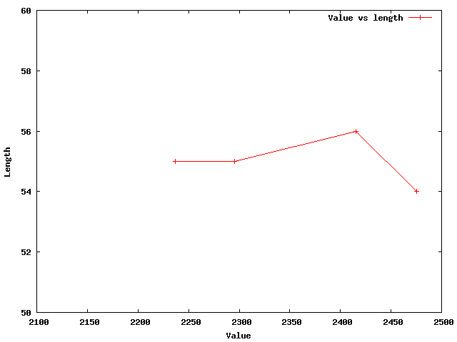
Since Gnuplot plots the points in ascending order, these values have to be read in reversed order, the first solution being the rightmost point and the last one being the leftmost one. If the same information would be needed but with the exact timings when each solution was generated, the following command makes the service:
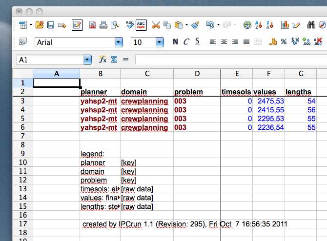
$ ./report.py --directory tempo-sat/ --variable timesols values lengths
              --planner yahsp2-mt --domain crewplanning --problem 003
              --unroll --style excel
This time, the report is generated in an Excel wordsheet named report.xls. A screenshot (generated with OpenOffice [10]) is shown below:
Ranking planners
It is usually a good idea, not only for the International Planning Competition, but also at the lab when conducting experiments with a number of planners to rank them according to their performance with regard to a particular set of planning tasks. The modules score.py (see score.py) and tscore.py (see tscore.py) are provided to get both an overall view and also a detailed picture of the performance of each planner in the results tree under consideration.
We start by showing a nice feature of the reporting tools. In all cases discussed in the previous subsection, the report.py module examined a given directory. It forced it to traverse the whole tree structure, visiting the directories of all the planning tasks to extract some information and then to back it up all the tree upwards. Because this tree contained only a few planners and domains, they could be processed very fast. However, if the tree gets large, this can result in an unecessary waste of time. To avoid it, summaries or snapshots can be generated instead —see Snapshots. These are just binary files that contain all the necessary information. Snapshots can be only generated by the module report.py. It suffices with requesting a report while specifing a snapshot filename as follows:
$ ./report.py --directory tempo-sat/ --variable numprobs
              --summarize tutorial.snapshot
Although only one variable has been specified, the resulting snapshot contains the values of all the acknowledged variables —see Reporting variables. Now, this snapshot can be used either by any of the modules in the package IPCReport. In this subsection, its usage is shown when ranking planners.
To rank planners using the metric used at the Seventh International Planning Competition with the snapshot previously generated [11]:
$ ./score.py --summary tutorial.snapshot

  ...

tempo-sat: crewplanning (Fri Oct  7 17:26:46 2011)
+-------+--------+-----------+---------+
|  no.  | yahsp2 | yahsp2-mt |   best  |
+-------+--------+-----------+---------+
|  000  |  1.00  |    1.00   | 2880.19 |
|  001  |  1.00  |    1.00   | 2880.20 |
|  002  |  1.00  |    1.00   | 2880.25 |
|  003  |  0.93  |    1.00   | 2236.54 |
|  004  |  1.00  |    1.00   | 1755.34 |
|  005  |  1.00  |    1.00   | 4320.39 |
|  006  |  1.00  |    1.00   | 4320.38 |
|  007  |  1.00  |    1.00   | 4320.48 |
|  008  |  1.00  |    1.00   | 3450.64 |
|  009  |  1.00  |    1.00   | 4230.97 |
|  010  |  1.00  |    1.00   | 5087.05 |
|  011  |  1.00  |    1.00   | 5087.16 |
|  012  |  1.00  |    1.00   | 5926.16 |
|  013  |  1.00  |    1.00   | 6706.43 |
|  014  |  1.00  |    1.00   | 7126.77 |
|  015  |  1.00  |    1.00   | 7486.85 |
|  016  |  1.00  |    1.00   | 3810.70 |
|  017  |  1.00  |    1.00   | 3990.76 |
|  018  |  1.00  |    1.00   | 4771.09 |
|  019  |  1.00  |    1.00   | 4337.25 |
| total | 19.92  |   20.00   |         |
+-------+--------+-----------+---------+

 ---: unsolved
  X : invalid

 created by IPCrun 1.1 (Revision: 295), Fri Oct  7 17:26:46 2011


tempo-sat: turnandopen (Fri Oct  7 17:26:46 2011)
+-------+--------+-----------+------+
|  no.  | yahsp2 | yahsp2-mt | best |
+-------+--------+-----------+------+
|  000  |   X    |     X     | ---  |
|  001  |   X    |     X     | ---  |
|  002  |   X    |     X     | ---  |
|  003  |   X    |     X     | ---  |
|  004  |   X    |     X     | ---  |
|  005  |   X    |     X     | ---  |
|  006  |   X    |     X     | ---  |
|  007  |   X    |     X     | ---  |
|  008  |   X    |     X     | ---  |
|  009  |   X    |     X     | ---  |
|  010  |   X    |     X     | ---  |
|  011  |  ---   |    ---    | ---  |
|  012  |   X    |     X     | ---  |
|  013  |   X    |     X     | ---  |
|  014  |   X    |     X     | ---  |
|  015  |   X    |     X     | ---  |
|  016  |   X    |     X     | ---  |
|  017  |   X    |     X     | ---  |
|  018  |   X    |     X     | ---  |
|  019  |   X    |     X     | ---  |
| total |  0.00  |    0.00   |      |
+-------+--------+-----------+------+

 ---: unsolved
  X : invalid

 created by IPCrun 1.1 (Revision: 295), Fri Oct  7 17:26:46 2011


tempo-sat: ranking (Fri Oct  7 17:26:46 2011)
+-----------+--------------+-------------+-------+
|  planner  | crewplanning | turnandopen | total |
+-----------+--------------+-------------+-------+
| yahsp2-mt |    20.00     |     0.00    | 20.00 |
|   yahsp2  |    19.92     |     0.00    | 19.92 |
|   total   |    39.92     |     0.00    |       |
+-----------+--------------+-------------+-------+

 ---: unsolved
  X : invalid

 created by IPCrun 1.1 (Revision: 295), Fri Oct  7 17:26:46 2011
As it can be seen, yahsp2-mt is slight better (according to the quality metric defined in the Seventh International Planning Competition) and should be preferred for those planning tasks that are similar to those used in this tutorial.
The same information can be generated in a LaTeX file that can be easily processed to get a pdf:
$ ./score.py --summary tutorial.snapshot --style latex
The resulting file is stored in a file named matrix.tex. This file cannot be processed with pdflatex since it uses the ps-tricks package. Instead, the IPCReport provides a makefile that can be used to generate the pdf:
$ make matrix.pdf
The resulting pdf file contains as many pages as domains have been found in the snapshot plus an additional one with an overall ranking table that summarizes all results. The following pictures show the three pages that are generated by the previous command:
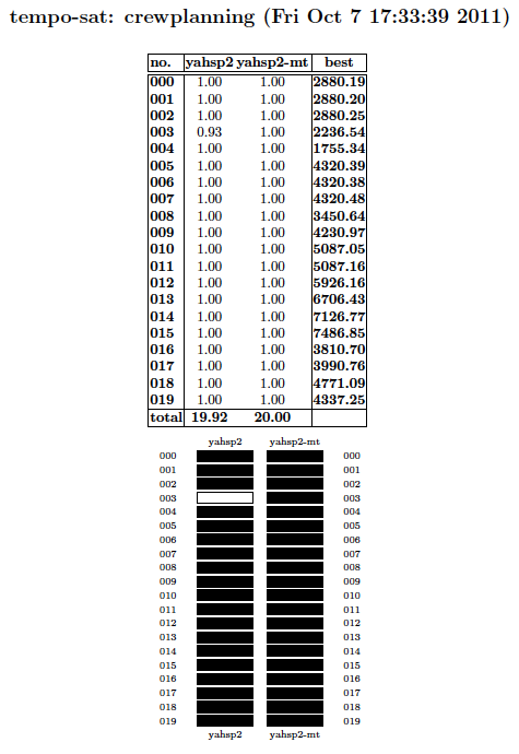
The first page shows the results in the crewplanning domain. The color codes used in the lower half represent the same information shown in the upper half but are easier to understand. The darker a box the better the performance; likewise, the lighter the box the worse. Here, better and worse are referred to the relative performance of each planner with respect to the others.
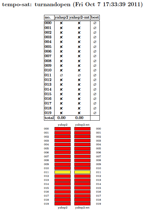
The second page shows the results in the turnandopen domain. In this case, the color codes are only either red or yellow. A red entry means that at least one plan was generated but that none was found valid. A yellow box means that no solution was generated for that particular problem.
In both cases, rows and columns are sorted lexicographically.
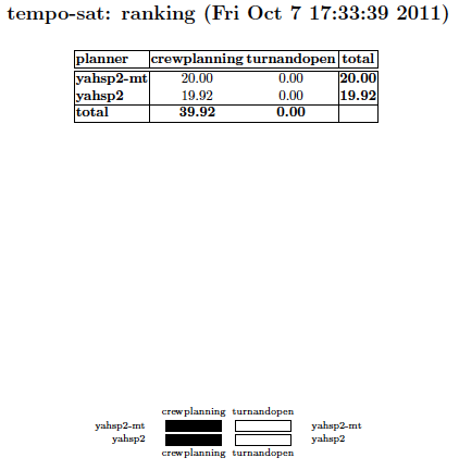
The third page provides an overall view of the performance of each planner in every domain. In this case, planners and domains are ranked in descending order of their total score. The color codes shown at the bottom follow the same notation discussed above.
Finally, a demo of the tscore.py is skipped since a full example is shown in tscore.py.
Second practical case
The second example shows how to set-up the environment for running experiments with the software developed at the Seventh International Planning Competition. This example has been explicitly created to encourage users to use this software for evaluating their own planners. The exercise consists of just creating a private svn server that will host just one planner and five problems of only one domain.
Creating the SVN repository
Before starting with this part of the tutorial, move to an empty ancilliary directory and make sure to follow all the steps depicted in Setting up but Configuring the IPC Software —if the external software described in those sections is already installed in your computer you can safely skip those steps. Next, create a new directory as follows:
$ cd ~/tmp
$ mkdir second-case
$ cd second-case
In this case two svn servers will be used at the same time: on one hand, the scripts will be retrieved from the official svn server of the Seventh International Planning Competition; on the other hand, a private svn server will be created to store an experimental planner and one testing domain. Therefore, if you decide to configure the IPC software as explained in Configuring the IPC Software make sure to use the following bookmark: file:///.../tmp/tutorial where the ellipsis should be replaced by the absolute path to your temporal directory [12] —more on this below.
First things first. This part of the tutorial will use the planner probe and the first five problems of the domain openstacks. The planner probe is known to have two specific requirements: makedepend and SCons so make sure to make them available in your GNU/Linux box:
$ sudo apt-get install xutils-dev
$ sudo apt-get install scons
Of course, it is expected that the user replaces this planner and domain by those of her choice but they are used here to make sure that they are available for private experimentation. Both are referred to the sequential satisficing (seq-sat) track of the Seventh International Planning Competition. Thus, it is mandatory to recreate in the local computer the same structure that shall be followed in the svn repository so that the IPC software can handle it —for more information see Contents of the data repository:
$ mkdir -p my-ipc/planners/seq-sat
$ mkdir -p my-ipc/domains/seq-sat
$ svn co svn://svn@pleiades.plg.inf.uc3m.es/ipc2011/data/planners/seq-sat/seq-sat-probe
      my-ipc/planners/seq-sat/seq-sat-probe
$ svn co svn://svn@pleiades.plg.inf.uc3m.es/ipc2011/data/domains/seq-sat/openstacks
      my-ipc/domains/seq-sat/openstacks
Before moving on, keep an eye on a very important issue. To make it feasible to automate both the building process of the planner and the creation of the testsets, the user has to provide to very important files: plan and build —for more details see check.py. The first one acts as a wrapper to command the planner to solve a particular problem in a particular domain. The second one shall fully automate the building process of the software. Make sure to:
- Prefix these scripts with appropriate shebang lines so that they can be executed
- Add all the necessary commands in plan to make your planner run in the desired mode
- Avoid your script build to use sudo command lines
These files are mandatory. Without them, the whole process will fail. It is the responsiblity of the programmer to provide them as the author of probe (Nir Lipovetzky) did here. When running your own example make sure to provide them. It might be a good idea to test these scripts locally before going any further.
Since we only want the first five problems of the domain openstacks, remove all the rest:
$ cd my-ipc/domains/seq-sat/openstacks
$ rm -rf domain/p06* domain/p07* domain/p08* domain/p09*
         domain/p1* domain/p2*
$ rm -rf problems/p06* problems/p07* problems/p08* problems/p09*
         problems/p1* problems/p2*
Finally, since all these files will go into a new repository, make sure to remove all the .svn subdirectories as follows:
$ cd ../../../
$ find . -name ".svn" -exec rm -rf \{\} \;
Now, everything is ready to create a new repository that will hold the selected planner and domain. First, create a svn repository called tutorial in your temporal directory as follows:
$ cd ~/tmp
$ svnadmin create tutorial
If you are not familiar with svn you are very welcome to examine the contents of this repository by browsing its directories. Bear in mind that this svn server is local and therefore will be accessed with the bookmark prefix file://. Since the path to it is .../tmp/tutorial (where the ellipsis stand for the absolute path to your home directory) a svn bookmark such as file:///.../tmp/tutorial results —note the three slashes after file: two are required by the svn prefix whereas the third one indicates the beginning of an absolute path. Now, check in the contents of my-ipc into the newly created repository [13]:
$ svn import second-case/my-ipc file:///home/clinares/tmp/tutorial -m "Initial import"
You are very welcome to browse the contents of your repository with svn list. For example:
$ svn list file:///home/clinares/tmp/tutorial
domains/
planners/
$ svn list file:///home/clinares/tmp/tutorial/domains
seq-sat/
You can inspect the contents of any directory in the repository just by adding it to the svn bookmark. Verify that the contents of your svn server are compliant with the arrangement described in Contents of the data repository.
Now that the svn repository has been created with the desired contents, you can safely remove your local directory:
$ rm -rf ~/tmp/second-case
Do not be scared! Its contents will be timely retrieved as shown below.
Testing the new SVN repository
The curious reader might want to try to automatically build the testsets of the domain stored in the new svn server or to automatically build the planner probe (while being in the directory where the package IPCData was checked-out):
$ ./buildplanner.py --track seq --subtrack sat --planner probe --directory ~/tmp
                    --bookmark file:///home/clinares/tmp/tutorial
$ ./builddomain.py --track seq --subtrack sat --domain openstacks --directory ~/tmp
                   --bookmark file:///home/clinares/tmp/tutorial
Note that this time a bookmark has been provided. The reason is that this svn server has not been configured as in the first practical case —see Configuring the IPC Software.
However, it is usually more practical to use the script invokeplanner.py instead as follows (if you typed in the previous two commands make sure to remove the directories ~/tmp/probe and ~/tmp/openstacks before proceeding):
$ ./invokeplanner.py --track seq --subtrack sat --planner probe --domain openstacks
                     --directory ~/tmp --bookmark file:///home/clinares/tmp/tutorial
                     --timeout 30 --memory 2
Since this svn server has not been configured, automatic notification by e-mail is not allowed. Instead, the log file will be shown on the standard output as the experiments progress —if the option --verbose is given, more information will be printed out. The information shown on the screen ends with a summary report of the number of problems solved and the number of plan solution files generated. In my computer (a rather old one), probe solved three of them generating up to 17 plan solution files.
Before making any queries to the results tree, validate all the results (make sure to have already installed in your system VAL 4.2.09 as discussed in Validating the results):
$ ./validate.py --directory ~/tmp/results/seq-sat
Next, a figure different than those shown in the first practical case is created here. To come out with the typical figure that shows the solving times and their corresponding quality two lines are about to be plot that represent the quality of the first and last solution at the corresponding times they are found. First, to make sure that the first solution is the worst one and, likewise, that the last solution is that the best one, command IPCReport to show up the qualities of all solutions found and the time stamps when they were computed [14]:
$ mv ../IPCReport
$ ./report.py --directory ~/tmp/results/seq-sat/ --variable timesols values --quiet
 name: report
+-----+---------+------------------------------+--------------------------------------------+
| ... | problem |           timesols           |                   values                   |
+-----+---------+------------------------------+--------------------------------------------+
| ... |   000   |    [6, 7, 10, 15, 22, 30]    |    [15.0, 14.0, 13.0, 12.0, 11.0, 10.0]    |
| ... |   001   |       [19, 21, 23, 25]       |          [24.0, 23.0, 22.0, 21.0]          |
| ... |   002   | [16, 18, 20, 22, 24, 26, 30] | [23.0, 22.0, 21.0, 20.0, 19.0, 18.0, 17.0] |
| ... |   003   |              []              |                     []                     |
| ... |   004   |              []              |                     []                     |
+-----+---------+------------------------------+--------------------------------------------+
 legend:
   planner [key]
   domain [key]
   problem [key]
   timesols: elapsed time when each solution was generated (in seconds) [raw data]
   values: final values returned by VAL, one per each *valid* solution file [raw data]

 created by IPCrun 1.2 (Revision: 295), Mon Oct 10 00:37:25 2011
Since this hyphotesis is satisfied (and should be satisfied always unless something goes really wrong!) create two octave files with the following commands:
$ ./report.py --directory ~/tmp/results/seq-sat/ --variable oktimefirstsol uppervalue --quiet
              --style octave > first.m
$ ./report.py --directory ~/tmp/results/seq-sat/ --variable oktimelastsol lowervalue --quiet
              --style octave > last.m
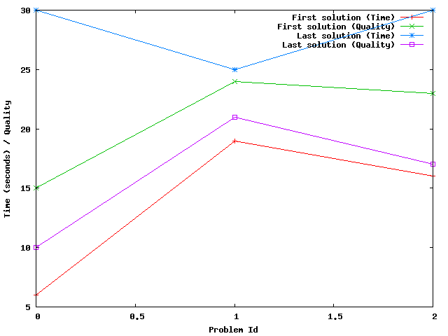
Remove the lines for the last two problems and now start a gnuplot session:
gnuplot> set xlabel "Problem Id"
gnuplot> set ylabel "Time (seconds) / Quality"
gnuplot> set terminal png
gnuplot> set output "timequality.png"
gnuplot> plot "first.m" using 3:4 with linesp title "First solution (Time)",
              "first.m" using 3:5 with linesp title "First solution (Quality)",
              "last.m" using 3:4 with linesp title "Last solution (Time)",
              "last.m" using 3:5 with linesp title "Last solution (Quality)"
The resulting image is shown below. It shows simultaneously both the time and quality of all the problems probe managed to solve:
Third practical case
The main goal of this exercise is to show how to perform comparisons among planners. To this end, we will use the results of the previous case to compare its performance with the winner of the Sequential Satisficing (seq-sat) track: lama-2011. In general, however, the same steps can be used to compare the performance of any planners in any set of domains. Therefore, this procedure can be used to make private experiments —for example, prior to the publication of a paper introducing a new planner.
After the preliminary experiments shown in the previous section, we will extend the experimentation to all problems in the openstacks domain. Therefore, before moving on make sure to follow the same procedure depicted before but without deleting any planning task. Instead, preserve all of them.
Getting the results tree directories
As it turned out in the previous case, we will be simultaneously using two different svn servers: one with the results of a private experimentation (that is exemplified in this case by experiments with probe) and another one with the results of an official entrant to the Seventh International Planning Competition.
As soon as a private server has been set-up (with the bookmark file://) named tutorial which contains only probe and all the planning tasks in the domain openstacks, obtain the new results tree structure as follows by running the module invokeplanner.py:
$ ./invokeplanner.py --track seq --subtrack sat --planner probe --domain openstacks
                     --directory ~/tmp --bookmark file:///home/clinares/tmp/tutorial
                     --timeout 30 --memory 2
Do not forget to validate these results using the module validate.py from the package IPCData:
$ ./validate.py --directory ~/tmp/results/seq-sat/probe/

 Revision: 296
 Date: 2011-10-06 01:16:57 +0200 (Thu, 06 Oct 2011)

 ./validate.py 1.1

 -----------------------------------------------------------------------------
 * directory : /Users/clinares/tmp/third-sat/probe
 -----------------------------------------------------------------------------

+---------------+----------+------------------+--------------------+
| # directories | # solved | # solution files | # successful plans |
+---------------+----------+------------------+--------------------+
|       20      |    4     |        23        |         23         |
+---------------+----------+------------------+--------------------+
As it can be seen this planner did not generate any invalid solution.
Now, retrieve from the official svn server of the Seventh International Planning Competition the results of lama-2011 in the same domain and store them in a separate directory of your temporal folder:
$ cd ~/tmp
$ mkdir -p ipc-sat/lama-2011
$ cd ipc-sat/lama-2011
$ svn co svn://svn@pleiades.plg.inf.uc3m.es/ipc2011/results/raw/seq-sat/lama-2011/openstacks
Two important remarks follow: first, when retrieving the results of lama-2011 in the openstacks domain they are stored in a directory which has to adhere to the conventions described in The results directory —here ipc and sat are the names of artificial tracks and subtracks; second, the results checked out from the official svn server are in raw format [15] so that they have to be validated before proceeding. Invoke the validation script from the module IPCData as follows:
$ ./validate.py --directory ~/tmp/ipc-sat

Revision: 296 Date: 2011-10-05 16:16:57 -0700 (Wed, 05 Oct 2011)

./validate.py 1.1

-----------------------------------------------------------------------------
* directory : /home/clinares/tmp/ipc-sat
-----------------------------------------------------------------------------

+---------------+----------+------------------+--------------------+
| # directories | # solved | # solution files | # successful plans |
+---------------+----------+------------------+--------------------+
|       20      |    20    |       187        |        187         |
+---------------+----------+------------------+--------------------+
Combining the results tree directories
Now, since the reporting scripts work from a unique results tree directory it is mandatory to merge both results tree directories into a separate one. In this example, it will be called third-sat.
First, start by populating third-sat with the contents of the results tree directory of lama-2011. To this end, move to the package IPCTools and execute the following command:
 $ ./copy.py --source ~/tmp/ipc-sat/lama-2011 --destination ~/tmp/third-sat

Revision: 296
Date: 2011-10-06 01:16:57 +0200 (Thu, 06 Oct 2011)

./copy.py 1.1

-----------------------------------------------------------------------------
* source      : ['/Users/clinares/tmp/ipc-sat/lama-2011']
* destination : /Users/clinares/tmp/third-sat
-----------------------------------------------------------------------------
The user is invited to inspect the contents of a particular problem in this artificial results tree directory:
$ cd ~/tmp/third-sat/lama-2011/openstacks/013
$ ls -lAF
total 1328
drwxr-xr-x  7 clinares  staff     238 Oct 11 16:09 .svn/
-rw-r--r--  1 clinares  staff    6826 Oct 11 16:09 _third-sat.lama-2011-openstacks.013-cpu
-rw-r--r--  1 clinares  staff   51202 Oct 11 16:09 _third-sat.lama-2011-openstacks.013-log
-rw-r--r--  1 clinares  staff    1266 Oct 11 16:09 _third-sat.lama-2011-openstacks.013-mem
-rw-r--r--  1 clinares  staff     873 Oct 11 16:12 _third-sat.lama-2011-openstacks.013-val
-rw-r--r--  1 clinares  staff     235 Oct 11 16:09 _third-sat.lama-2011-openstacks.013-ver
-rw-r--r--  1 clinares  staff   65513 Oct 11 16:09 build-lama-2011.log
-rw-r--r--  1 clinares  staff   94228 Oct 11 16:09 domain.pddl
-rw-r--r--  1 clinares  staff   14384 Oct 11 16:09 plan.soln.1
-rw-r--r--  1 clinares  staff   14357 Oct 11 16:09 plan.soln.2
-rw-r--r--  1 clinares  staff   14168 Oct 11 16:09 plan.soln.3
-rw-r--r--  1 clinares  staff   14141 Oct 11 16:09 plan.soln.4
-rw-r--r--  1 clinares  staff   14114 Oct 11 16:09 plan.soln.5
-rw-r--r--  1 clinares  staff       0 Oct 11 16:09 planner.err
-rw-r--r--  1 clinares  staff  319586 Oct 11 16:09 planner.log
-rw-r--r--  1 clinares  staff   36603 Oct 11 16:09 problem.pddl
As it can be seen, the files have been conveniently renamed to make them look as if they were originally created under a track/subtrack named third-sat.
Next, extend the contents of this results directory by copying there the results obtained with the planner probe:
 $ ./copy.py --source ~/tmp/results/seq-sat/probe --destination ~/tmp/third-sat

Revision: 296
Date: 2011-10-06 01:16:57 +0200 (Thu, 06 Oct 2011)

./copy.py 1.1

-----------------------------------------------------------------------------
* source      : ['/Users/clinares/tmp/results/seq-sat/probe']
* destination : /Users/clinares/tmp/third-sat
-----------------------------------------------------------------------------
Now, third-sat contains the results of two planners:
$ dir ~/tmp/third-sat/
total 0
drwxr-xr-x  3 clinares  staff  102 Oct 11 16:09 lama-2011/
drwxr-xr-x  3 clinares  staff  102 Oct 11 15:59 probe/
for one particular domain:
$ dir ~/tmp/third-sat/lama-2011
total 0
drwxr-xr-x  23 clinares  staff  782 Oct 11 16:09 openstacks/
$ dir ~/tmp/third-sat/probe
total 0
drwxr-xr-x  22 clinares  staff  748 Oct 11 16:11 openstacks/
Accessing the new results tree directory
Finally, with a unique results tree directory containing the results of the planners of choice with regard to the selected domains of interest it is possible to access the results with the reporting tools in the package IPCReport.
In the following example, the results tree directory third-sat is directly accessed —i.e., no snapshot is generated. In this case we will require the reporting tools to show information on the number of problems solved and those where the planner failed:
 $ /report.py --directory ~/tmp/third-sat/ --variable numsolved oknumsolved numtimefails nummemfails
              --level planner

Revision: 297
Date: 2011-10-06 16:22:31 +0200 (Thu, 06 Oct 2011)

./report.py 1.2

  -----------------------------------------------------------------------------
  * directory      : /Users/clinares/tmp/third-sat
  * snapshot       :
  * name           : report
  * level          : planner
  * planner        : .*
  * domain         : .*
  * problem        : .*
  * variables      : ['numsolved', 'oknumsolved', 'numtimefails', 'nummemfails']
  * unroll         : False
  * sorting        : []
  * style          : table
  -----------------------------------------------------------------------------

  name: report
 +-----------+-----------+-------------+--------------+-------------+
 |  planner  | numsolved | oknumsolved | numtimefails | nummemfails |
 +-----------+-----------+-------------+--------------+-------------+
 | lama-2011 |     20    |      20     |      0       |      0      |
 |   probe   |     4     |      4      |      16      |      0      |
 +-----------+-----------+-------------+--------------+-------------+
 ...

  created by IPCrun 1.2 (Revision: 295), Tue Oct 11 16:53:45 2011
From the preceding table it follows that while lama-2011 solved all instances, probe only managed to solve four failing on time on all the rest. This is not surprising taking into account that these experiments were performed allowing probe to run only for 30 seconds per instance while lama-2011 was given 30 minutes in the Seventh International Planning Competition.
Fourth practical case
In this practical case we want to know whether one sequential satisficing planner, yahsp2, performs better than its multithreaded version, yahsp2-mt, for solving a particular case: problem 001 of the domain openstacks of the sequential satisficing track.
The hypothesis set in this experiment are the following:
Null Hypothesis: Both planners perform much alike and the mean time to generate solutions is the same. Alternate Hypothesis: One planner performs better than the other and tend to produce solutions faster.
The precise moments in time when both planners provided solutions can be found with the script report.py as follows [16]:
$ ./report.py --summary ./seq-sat.results.snapshot --variable timesols
              --domain openstacks --problem 001 --planner 'yahsp2'
Both series can be automatically retrieved by the script test.py using exactly the same parameters. However, it only accepts single-valued series so that the argument --unroll should be provided as well. test.py creates automatically two series from the results provided by report.py, one with the exact timings of all the solutions found by yahsp2 and another for yahsp2-mt. This is done automatically because the leftmost column of the report obtained with the previous command (which is planner) contains the names of the series of interest: yahsp2 and yahsp2-mt.
By simple inspection of the results of the previous report it seems that yahsp2 tends to take longer to provide solutions yet, it produces 33 solutions, while yahsp2-mt seems to be faster but solving almost ten problems less [17]. The non-parametrical statistical test Mann Whitney U test can be used for this purpose. It just suffices to invoke it with the same parameters than above (and --unroll as already discussed) and --test mw to specify this particular test:
$ ./test.py --summary ./seq-sat.results.snapshot --variable timesols
            --domain openstacks --problem 001 --planner 'yahsp2' --unroll
            --test mw

   Revision
   Date

   ./test.py 1.3

   -----------------------------------------------------------------------------
   * snapshot       : ./seq-sat.results.snapshot
   * tests          : ['Mann-Whitney U']
   * name           : report
   * level          : None
   * planner        : yahsp2
   * domain         : openstacks
   * problem        : 001
   * variable       : ['timesols']
   * filter         : None
   * matcher        : all
   * noentry        : -1
   * unroll         : True
   * sorting        : []
   * style          : table
   -----------------------------------------------------------------------------


   name: report
  +-----------+-------------------+-------------------+
  |           |       yahsp2      |     yahsp2-mt     |
  +-----------+-------------------+-------------------+
  |   yahsp2  |        ---        | 2.43846017451e-05 |
  | yahsp2-mt | 2.43846017451e-05 |        ---        |
  +-----------+-------------------+-------------------+
   Mann-Whitney U : Computes the Mann-Whitney rank test on two samples. It assesses whether one of two samples of
   independent observations tends to have larger values than the other. This test corrects for ties and
   by default uses a continuity correction. The reported p-value is for a one-sided hypothesis, to get
   the two-sided p-value multiply the returned p-value by 2.

   created by IPCtest 1.3 (Revision: 312), Sun Jul 15 23:40:18 2012
The preceding table reports a p-value equal to 0.0000243 that one serie tends to have larger values than the other. Since this is the p-value of the one-sided hypothesis, the Null Hypothesis can be discarded even with a confidence level of α=0.001 (i.e., with a probability of 99.9% that the difference are real and not due to chance) and the Alternate or Research Hypothesis that yahsp2-mt is faster can be accepted.
For more information about this script see section test.py where another case with more options is discussed in depth.
Before finishing, this script acknowledges all the different styles provided by report.py with the directive --style so that the same tables can be shown in the markup languages html and wiki, Octave files and also in excel worksheets.
Note
To know more about their relative performance in these domain and others as well as performing comparisons with a large number of planners (including some programmed by you or your colleagues) you are invited to start using the software of the Seventh International Planning Competition.
Footnotes
| [1] | While Python also provides a wrapper for accessing INI configuration files, this was found to be very complete and easy to deal with. |
| [2] | The current version of ConfigObj at the time of writing this tutorial was 4.7.2. Obviously, the directory to step in might change if new versions have been deployed later. |
| [3] | Also, the so-called svn-workbench is distributed from the same homepage (and it is also available as an Ubuntu package). However, it is not needed at all for using the IPC software. |
| [4] | The current version of pyExcelerator at the time of writing this tutorial was 0.6.4.1. Obviously, the directory to step in might change if new versions have been deployed later. |
| [5] | Most readers can find this valuable. An image of the official svn server can be requested by e-mail to carlos.linares@uc3m.es. Then, its contents can be recreated in a private svn server where a number of experiments can be conducted without letting others notice. |
| [6] | Note that because planners and domains are distinguished by the track/subtrack they belong to, planners and domains in differen tracks/subtracks can be named the same. |
| [7] | This actually means that one could download domains from one svn server and planners from a different one. To override the default selection set in the INI configuration file it suffices with specifying a new svn bookmark with the --bookmark directive |
| [8] | Other names can be used with the option --logfile |
| [9] | Besides, the building process complies about a number of autotools. But these are not required (as informed by the warning message issued) unless the Makefile.am is likely to change and that is not the case here. |
| [10] | Nowadays, LibreOffice is a nice alternative to OpenOffice. |
| [11] | These tables were inspired by a very similar ones that were automatically generated in the Sixth International Planning Competition. |
| [12] | In my case this would be /home/clinares so that the whole svn bookmark reads as file:///home/clinares/tmp/tutorial and it should be pretty similar in all cases. |
| [13] | /home/clinares has been added for the sake of clarity but the absolute path to your temporal directory shall replace it |
| [14] | The first two columns have been ommitted to make the whole table fit the width of the LaTeX version of this manual |
| [15] | As a matter of fact, it is feasible instead to check out the validated contents from the directory val instead of raw. However, it is highly recommended to download always the raw results and to validate them locally. |
| [16] | The output is not shown because it exceeds the right margin of this document |
| [17] | The reader is warned that all these solutions were found invalid by VAL so that the variables to use here will refer to the values of interest not validated by VAL. |